library("dplyr")
Attaching package: 'dplyr'The following objects are masked from 'package:stats':
filter, lagThe following objects are masked from 'package:base':
intersect, setdiff, setequal, unionlibrary("ggplot2")library("dplyr")
Attaching package: 'dplyr'The following objects are masked from 'package:stats':
filter, lagThe following objects are masked from 'package:base':
intersect, setdiff, setequal, unionlibrary("ggplot2")Control structures in R provide conditional flow as well as looping. An R expression is evaluated within the loop or as the result of a conditional statement.
The following are example R expressions
# First expression
1+2
[1] 3# Second expression
a <- 1; b <- 2; a+b[1] 3# Third expression
{
a <- 1
b <- 2
a + b
}[1] 3See
?expressionConditionals include if-else type statements
# Example (boring) if statement
if (TRUE) {
  print("This was true!")
}
[1] "This was true!"# if() using variable
this <- TRUE
if (this) {
print("`this` was true!")
}[1] "`this` was true!"# if() with comparison
if (1 < 2) {
print("one is less than two!")
}[1] "one is less than two!"if (1 > 2) {
print("one is greater than two!")
}Using variables
# Assign values
a <- 1
b <- 2

# Compare values
if (a < 2) {
  print("`a` is less than 2!")
}
[1] "`a` is less than 2!"if (a < b) {
print("`a` is less than `b`!")
}[1] "`a` is less than `b`!"# Example using if-else
if (a < b) {
  print("`a` is less than `b`!")
} else {
print("`b` is not less than `a`!")
}[1] "`a` is less than `b`!"# Second example
if (a > b) {
print("`a` is greater than `b`!")
} else {
print("`a` is not greater than `b`!")
}[1] "`a` is not greater than `b`!"You can use multiple if-else statements.
# Example of multiple else statements
if (a > b) {
  print("`a` is greater than `b`!")
} else if (dplyr::near(a,b)) {
  print("`a` is near `b`!")
} else {
  print("`a` must be greater than b")
}
[1] "`a` must be greater than b"Incorporate these statements into a function makes things more interesting.
# Function with if statements
compare <- function(a, b) {
  if (a > b) {
    print("`a` is greater than `b`!")
  } else if (dplyr::near(a,b)) {
    print("`a` is near `b`!")
  } else {
    print("`a` must be greater than b")
  }
}

# Use function
compare(1, 1)
[1] "`a` is near `b`!"compare(1, 2)[1] "`a` must be greater than b"compare(2, 1)[1] "`a` is greater than `b`!"compare(sin(2*pi), 0)[1] "`a` is near `b`!"The ifelse() function takes a logical vector as a first argument and then two scalars.
# Examples of ifelse
ifelse(c(TRUE, FALSE, TRUE),
       yes = "this was true",
       no  = "this was false")
[1] "this was true" "this was false" "this was true" # Vectorized yes/no
ifelse(c(TRUE, FALSE, TRUE),
yes = c( "true1", "true2", "true3"),
no = c("false1", "false2", "false3"))[1] "true1" "false2" "true3" A common usage of ifelse() is in data wrangling. For example, suppose you wanted to change cut levels Ideal and Premium to a category called Best.
# Examples of ifelse within mutate
d <- ggplot2::diamonds |>
  mutate(
    # Create new variable
    cut_new = ifelse(cut %in% c("Ideal", "Premium"),
                     "Best",
                     "Not Best"),

    # Overwrite existing variable
    cut = as.character(cut),
    cut = ifelse(cut %in% c("Ideal", "Premium"),
                 "Best",
                 cut), # replace with existing value of `cut`
    cut = factor(cut)
  )

# Check results
table(d$cut)
     Best      Fair      Good Very Good
35342 1610 4906 12082 table(d$cut_new)
    Best Not Best
35342 18598 A rarely used function is switch() which implements a case-switch comparison.
# Examples of switch
this <- "a"
switch(this,
       a = "`this` is `a`",
       b = "`this` is `b`",
       "`this` is not `a` or `b`")
[1] "`this` is `a`"this <- "b"
switch(this,
a = "`this` is `a`",
b = "`this` is `b`",
"`this` is not `a` or `b`")[1] "`this` is `b`"this <- "c"
switch(this,
a = "`this` is `a`",
b = "`this` is `b`",
"`this` is not `a` or `b`")[1] "`this` is not `a` or `b`"There are 3 base types of loops: for, while, and repeat. In addition, there is a convenience function replicate that allows us to easily repeatedly execute an R expression. This function is very useful for simulation studies.
The most common use of a for loop is to loop over integers.
# Loop over integers
for (i in 1:10) {
  print(i)
}
[1] 1
[1] 2
[1] 3
[1] 4
[1] 5
[1] 6
[1] 7
[1] 8
[1] 9
[1] 10for (j in 0:-10) { # can use any R name as iterator
print(j)
}[1] 0
[1] -1
[1] -2
[1] -3
[1] -4
[1] -5
[1] -6
[1] -7
[1] -8
[1] -9
[1] -10It is extremely common to utilize conditionals within a loop.
# Loops with if
for (i  in 1:10) {
  if (i > 5)
    print(i)
}
[1] 6
[1] 7
[1] 8
[1] 9
[1] 10for (i in 1:10) {
if (i %% 2) # mod function, implicit logical
print(i)
}[1] 1
[1] 3
[1] 5
[1] 7
[1] 9We can also iterate over non-integers by using any vector as the iterated values.
# Loop over numbers
for (i in c(2.3, 3.5, 4.6)) {
print(i)
}[1] 2.3
[1] 3.5
[1] 4.6# Loop over character
for (i in letters[1:5]) {
print(i)
}[1] "a"
[1] "b"
[1] "c"
[1] "d"
[1] "e"# Loop over strings
for (c in c("my","char","vector")) {
print(c)
}[1] "my"
[1] "char"
[1] "vector"# Loop over factor
for (i in unique(warpbreaks$tension)) {
print(paste(i, is.factor(i)))
}[1] "L FALSE"
[1] "M FALSE"
[1] "H FALSE"While these other
seq_along()Be careful when iterating over objects that a potentially NULL.
# Loop over 0 length vector
this <- NULL
for (i in 1:length(this)) {
print(i)
}[1] 1
[1] 0Since this had no length, you probably didn’t want to enter the for loop at all. To be safe, you can use seq_along().
# Use seq-along
for (i in seq_along(this)) {
print(i)
}my_chars <- c("my","char","vector")
for (i in seq_along(my_chars)) {
print(paste(i, ":", my_chars[i]))
}[1] "1 : my"
[1] "2 : char"
[1] "3 : vector"seq_len()For data.frames use seq_len() with nrow().
# seq_len() with nrow()
for (i in seq_len(nrow(ToothGrowth))) {
if (ToothGrowth$supp[i] == "OJ" &
near(ToothGrowth$dose[i], 2) &
ToothGrowth$len[i] > 25) {
print(ToothGrowth[i,])
}
} len supp dose
51 25.5 OJ 2
len supp dose
52 26.4 OJ 2
len supp dose
56 30.9 OJ 2
len supp dose
57 26.4 OJ 2
len supp dose
58 27.3 OJ 2
len supp dose
59 29.4 OJ 2Like with if and else statements, for loops can omit the brackets { } for single line expressions.
# for without {}
for (i in 1:10)
print(i)[1] 1
[1] 2
[1] 3
[1] 4
[1] 5
[1] 6
[1] 7
[1] 8
[1] 9
[1] 10The while() loop can be used to construct while loops.
# Example while loop
a <- TRUE
while (a) {
  print(a)
  a <- FALSE
}
[1] TRUETypically, you will have a conditional statement within the loop that will set the argument to FALSE.
# while example as a for loop
i <- 0
while (i < 10) {
  print(i)
  i <- i + 1
}
[1] 0
[1] 1
[1] 2
[1] 3
[1] 4
[1] 5
[1] 6
[1] 7
[1] 8
[1] 9We will only enter the loop if the argument to while is TRUE the first time.
# Evaluated before the loop
x <- 2
while (x < 1) {
  print("We entered the loop.")
}

# Evaluated after each loop
while (x < 100) {
  x <- x*x
  print(x)
}
[1] 4
[1] 16
[1] 256These loops will run until the argument in the while() function evaluates to FALSE. If this doesn’t occur, you have an infinite loop. To exit and infinite loop, use the ESC key.
while (TRUE) {
  # do something
}
Often, you will want to make sure the infinite loop never occurs. You can do this by counting the number of iterations of the loop and limiting how many iterations can be executed.
max_iterations <- 1000
i <- 1
while (TRUE & (i < max_iterations) ) {
  i <- i + 1
  # Do something
}
print(i)
[1] 1000An alternative to while() is repeat combined with break.
# repeat break
i <- 10
repeat {
  print(i)
  i <- i + 1
  if (i > 13)
    break
}
[1] 10
[1] 11
[1] 12
[1] 13Using next allows you to go to the next iteration of the repeat statement rather than breaking out of it.
i <- 1
repeat {
print(i)
i <- i + 1
if (i %% 2) { # %% is the mod function, 0 is FALSE and 1 is TRUE
next # skips to next iteration of repeat
}
if (i > 14)
break
}[1] 1
[1] 2
[1] 3
[1] 4
[1] 5
[1] 6
[1] 7
[1] 8
[1] 9
[1] 10
[1] 11
[1] 12
[1] 13
[1] 14
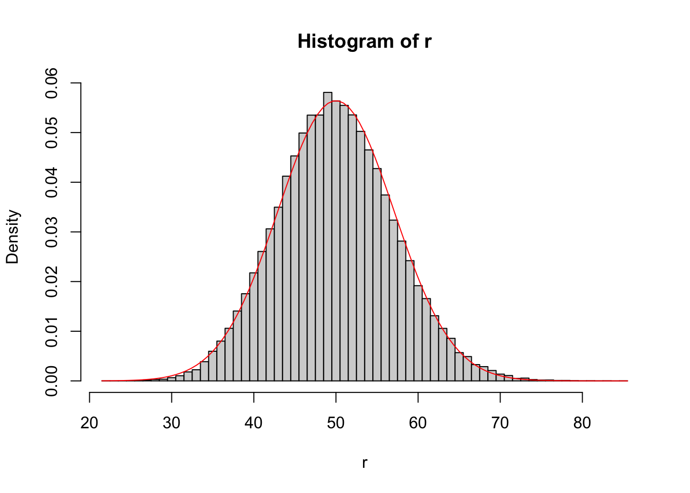
[1] 15The replicate function allows you to repeatedly execute an R expression. This can be handy in simulation studies.
# Demonstrate Central Limit Theorem for Poisson
n    <- 10
rate <- 5
r <- replicate(1e5, {       # number of replicates
  sum(rpois(n      = n,
            lambda = rate))
})

# Histogram of simulation draws
hist(r,
     breaks = seq(
       min(r) - 0.5,
       max(r) + 0.5,
       by = 1),
     prob = TRUE)

# Add CLT approximation
curve(dnorm(x,
            mean = n*rate,
            sd   = sqrt(n*rate)),
      add = TRUE,
      col = "red")
Despite only have \(n=10\), the CLT approximation is quite good because the CLT scales with the product of \(n\) and the Poisson rate.
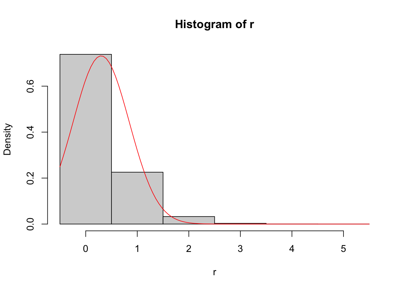
# Demonstrate CLT for binomial
n <- 30
p <- 0.01
r <- rbinom(1e5, size = n, prob = p) # no need for replicate

# Histogram of simulation draws
hist(r,
     breaks = seq(
       min(r) - 0.5,
       max(r) + 0.5,
       by = 1),
     prob = TRUE)

# Add CLT approximation
curve(dnorm(x,
            mean = n*p,
            sd   = sqrt(n*p*(1-p))),
      add = TRUE,
      col = "red")
This approximation is terrible since the CLT scales with \(n\times p\) rather than simply \(n\).